Sampling Errors

Sampling Error & Confidence Intervals

Another step-in data preparation is testing for sampling errors. 

When research is conducted a sample (n) is taken from the wider population (N). Who takes part in the research depends on the sampling technique used. There are many different sampling techniques all with different advantages and disadvantages, statistical testing relies on random sampling techniques. Whilst there are different types of random sampling techniques none are perfect and there is always the potential for anomalies to affect analysis. When this occurs, this can be due to a sampling error but this is something we can test for before doing any analysis so these errors have limited potential to affect our analysis. 

It’s important to test for sampling errors as these being present in our data could mean we come to a false conclusion during analysis. It could result in us either accepting or rejecting our hypothesis when the opposite is actually true, we could potentially have what is known as a: 

Type I error: occurs when a null hypothesis is rejected when its true (false positive) 

OR

Type II error: occurs when the null hypothesis is accepted when it is not true (false negative) 

We need to establish confidence in our sample, that our sample is representative of the wider population. We establish a confidence level by using the following steps. 

To demonstrate these steps, we will continue to use the cut-down version of Opinion Lifestyle Dataset 2015. Using this dataset, we will explore male and female life satisfaction. 

We want to make sure our data (for males and females) is from the same sample, to test for this we simply review a box and whisker plot.

To produce a box and whisker plot in R studio we use the command 

boxplot(opintfd$’LifeSat’~ opintfd$Gender)

A box plot should be produced in the bottom right panel, if an error message like the one shown in the console appears and the bottom right features the ‘figure margins too large’ message you just need to adjust your panels enlarging the bottom right so the box plot can fit. 

Having adjusted the panel margins we can see the box plot for Gender and Life Satisfaction. 

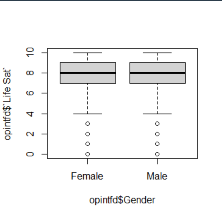
If we can draw a line that overlaps the two (or sometimes more) sample groups as shown above, then we can be confident that in this case our two groups are from the same sample.

The boxes indicate the range of scores that make up the mean and what our example shows is the difference between the two groups, we can just about see that the female mean is higher than the male mean, this may indicate a gender difference. This is what we would then go on to test. 

How to present your findings…

‘A review of a box and whisker plot (see figure ?) suggested that the data was free from sampling errors. For males, the mean 7.64 (CIs = 7.51-7.77), females, the mean =7.69 (CIs= 7.58-7.81), demonstrating that the mean is representative of the wider population.’

1. Education and Life Satisfaction (enter findings below)

1. Ethnicity and Life Satisfaction (enter findings below)