


In this guide we will be learning how to conduct Tests for Difference, when comparing more than two groups. The purpose of this guide is to expand your understanding of tests for difference beyond comparing only dichotomous variables.
This guide will help you in completing other RISE intensives, such as those for other Bivariate analysis tests.
Step 1 – Accessing the data
The data we are going to analyse is a cutdown dataset from the Opinions and Lifestyle Survey: Well-Being Module, 2015. This is the same dataset we’ve been using throughout this Rise course so it should already be saved in a secure folder. Details about the study can be found online at shorturl.at/mtyCZ.
Steps: Run SPSS > click open another file > Find relevant file > open into SPSS > the dataset should then load into the SPSS Variable View window.
These steps are also illustrated in screenshots below.


Your data should look like the screenshot below, especially if you’ve been following the steps in previous sprints. The data shown below has been cleaned and one variable ‘Employment2’ is an example of recoding.
This screenshot shows a customized variable view, if you haven’t already done so to customise your own, go to view >customize variable view, you only need the columns shown below.

Step 2 – Data Preparation
Data preparation for Tests for Difference was explored in a previous intensive so we won’t repeat these steps here. However, it’s worth remembering that you need to always:
- Explore data through descriptive statistics
- Create hypotheses
- Identify levels of measurement for variables
- Clean your data.
- Recode variables where necessary.
- Identify most suitable test for measurement type & hypothesis
- Test for Sampling Error and confidence.
Again, this has all been outlined in previous guides.
Step 3- Testing for Parametric Assumptions in Tests for Difference
Before running any parametric tests in tests for difference, your data must meet three different conditions. If data fails to meet parametric assumptions and therefore violates these assumptions a non-parametric test must be selected instead. Ideally a parametric test would be used as they’re stronger, more robust and any results carry more weight than non-parametric test. But if data does end up violating one or more assumptions a non-parametric test will simply be chosen instead.
You’ve already learnt how to do t-test and Mann-Whitney, but what happens when you want to use an IV with more than two groups?
We need some more groups in here…
t-test and Mann-Whitney are only useful when comparing variables with two groups, but many research questions require us to examine multiple groups (2+) at a time, when we want to have more than 2, we employ different statistical tests. When comparing 2+ groups the parametric test is ANOVA and non-parametric is a Kruskal-Wallis test.
As a reminder the three parametric assumptions are:
1. The dependent variable must be measured at the Interval level (Scale/Ordinal) and the
independent variables must be measured at the Categorical level.
2. Be normally distributed
3. Be of equal variance (homogeneity)
This has all already been outlined in a previous intensive, so we won’t repeat these steps here. If you need to remind yourself of how to conduct parametric assumption testing, go back to the previous intensive in this course.
Testing for Difference: Comparing 2+ Groups
Example
Suppose we wanted to explore the factors that are linked to British people’s life satisfaction, in our dataset we have numerous different variables which we could test (for difference) against the scale DV of Life Sat. We want to solely focus on the variables which have more than 2 groups so: Education, Employment and Age are our only possible IVs.
Research Question: Do British people’s level of life satisfaction differ by age?
Null Hypothesis: British people’s level of life satisfaction does not differ by age
Research Hypothesis: British people’s level of life satisfaction does differ by age
Variables and level of measurement
DV (Interval Scale): Life Satisfaction measured on a scale.
IV (Categorical Ordinal): Age measured across 4 groups.
The data was examined first to see if it met parametric assumptions, again these steps won’t be conducted here as they’ve already been outlined. The data was found to meet parametric assumptions thus an ANOVA was selected for further analysis.
Use ANOVA ONLY if data fulfils the conditions for both normality and homogeneity of variance. If one or more parametric assumptions is violated use Kruskal-Wallis.
Running an ANOVA in SPSS
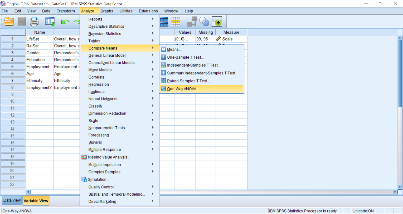
Select Analyze > Compare means > One-Way ANOVA
A box will open, place the dependant variable LifeSat in dependent list and the IV Age under factor.
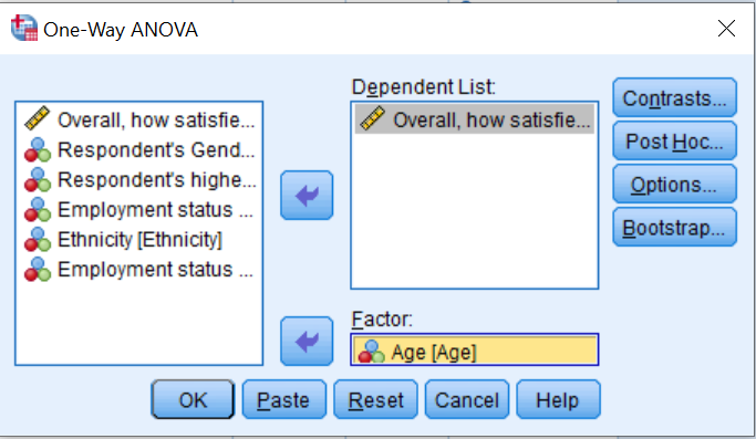
Select Options. Tick descriptives and press continue and OK. After this the ANOVA outputs should be produced.

Interpreting ANOVA results.

Highlighted we can see the mean life satisfaction score for the different age groups.

Looking at the Sig. we need to compare it with the threshold value of 0.05. If the significance is less than 0.05 we reject our null hypothesis. And this would mean the findings of our study provide evidence to suggest that British people’s level of life satisfaction differs by age. We can see that our sig. value is less than 0.05 we would therefore reject the null hypothesis, this suggests that life sat does differ by age.
The statistical significance of the F- test tell us the level of life sat significantly differs by age group. However, the test conducted does not tell us which groups differ from which. It’s therefore necessary after conducting an ANOVA and finding significance to carry out further analysis to find out which groups differ.
Conducting post hoc tests.
Following the steps above to conduct an ANOVA. When you get to this point you must select the ‘post hoc’ test function and a dialogue box will appear.

There are a number of post hoc tests to choose from. You need to select ‘Scheffe’ test if you have an unequal sample size for each group of the (nominal) variable in your hypothesis. If group size is equal, select ‘Tukey’ test. In our hypothesis, the sample size for each age group is unequal. Therefore, we have chosen the Scheffe test. Then click ‘continue’ and then OK.
Below are the test results on differences in life satisfaction amongst different age groups. We need to look at the significance level values to decide whether a group differs significantly from others or not. For example, three significance values (.735, .923,.920) in the highlighted box are for the difference between ‘16-24 and 25-44’, ’16-24 and 45-64’ and 16-24 and 65+’, none of these are statistically significant as they’re all larger than the threshold value of 0.05.

All of the significance values for each group need to be examined (16-24, 25-44, 45-64 and 65+) as well to find out whether there are any values less than 0.05. Reviewing the table, we can see for the age group 25-44 we find one value significant (.017). This is for the comparison between age group ’25-44’ and ’45-64’
As we used a two-tailed hypothesis the null hypothesis would be rejected. But as can be seen from the post-hoc tests only one combination between the groups is significant
25-44 and 45-64- significance p<.017.
Presenting findings
We would report all of these findings as the following:
An independent one-way ANOVA found a significant different between life satisfaction and age group (F=4.171, df=3, p=.006). We therefore reject the null hypothesis. This study provides evidence to suggest that British people’s life satisfaction differs by age group.
Further analysis by post hoc tests found a statistically significant difference (p=.017) in levels of life satisfaction between the 25-44 and 45-64 age groups.
There were no significant differences found in levels of life satisfaction between any of the other age groups.
Below is a how-to video of the steps we have just covered!
Running a Non-Parametric Kruskal-Wallis test
Research Question: Do British people’s level of life satisfaction differ by employment status?
Null Hypothesis: British people’s level of life satisfaction does not differ by employment status.
Research hypothesis: British people’s level of life satisfaction does differ by employment status.
Variables and level of measurement:
DV (Interval Scale): Life Satisfaction measured on a scale.
IV (Categorical Nominal): Employment status with 3 categories.
The data was examined first to see if it met parametric assumptions, again these steps won’t be conducted here as they’ve already been outlined.
The data was tested prior to further analysis and was found to violate parametric assumption for homogeneity, data was found to be heterogenous so a non-parametric test Kruskal-Wallis was selected for further analysis.
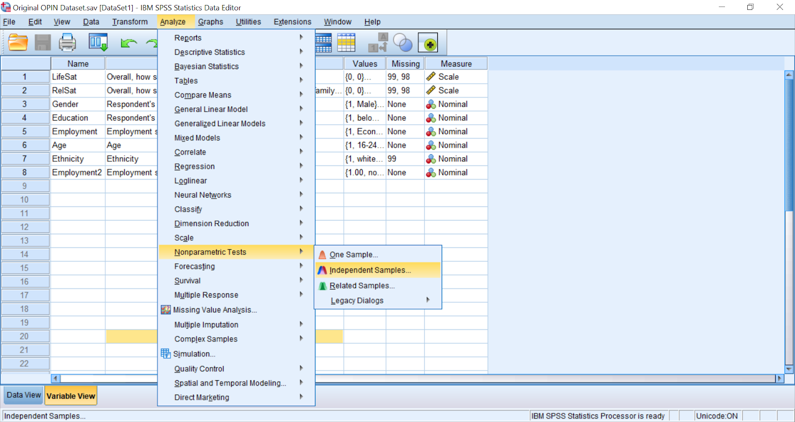
Select Analyze > Nonparametric test > Independent Samples.
A box will open, under what is your objective ‘Automatically compare’ will be pre-selected, change this default setting to custom analysis.

Click > Fields. Here you will insert your scale DV Life Sat into ‘Test fields’ and the nominal IV employment status into ‘Groups’

Then click > Settings. This will take you to the screen shown below. Make sure you’ve chosen > customise tests, select > Kruskal-Wallis and > ‘All pairwise’ in the dialogue box. Then click > run to get the results.

Interpreting Kruskal-Wallis test.

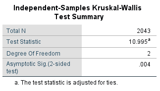
In the SPSS output screen this box above will appear, it shows a summary of results. It shows the significance value for the test, as well as he decision you need to make (to reject the null hypothesis in this case). This study provides evidence to suggest that British people’s life satisfaction differs by employment status.
The test has produced a few other outputs which provide further insight.

The higher the mean rank indicates a greater level of life satisfaction. The economically inactive appear to have the highest mean level of Life Sat.
When you reject the null hypothesis as we’ve done here you need to conduct further analysis (as you did for ANOVA) this is done so we know which groups differ significantly. SPSS has done this for you as well.


We’re concerned with the adjusted sig value here. If any of these values are less than 0.05 then group differences are statistically significant. As we chose a two-tailed test for significance we can remain using 0.05 but f you want to do a one-tailed test of significance, use 0.025 (0.05/2) as threshold value (instead of 0.05) and compare this with ‘Adjusted Sig’ values and make the decision.
In this example we see that two pairs of comparison are statistically significant (.031 and .005) as they’re less than the threshold for a two-tailed hypothesis. Therefore we can say that ILO unemployed have a statistically significant lower level of happiness compared to the other employment status’.
Presenting findings
The results of the Kruskal-Wallis test (H=10.995, df=2, p=.004) found a statistically significant difference between British people’s level of life satisfaction and their employment status. We, therefore reject the null hypothesis.
Further analysis by pairwise comparison tests found significant differences in British people’s level of life satisfaction across 1 employment status. A significant difference (p=.031) was found in level of life satisfaction between ILO unemployed (mean rank = 833.34) and In employment (mean rank =1010.37) and a significant difference (p=.005) between ILO unemployed and the economically inactive (mean rank =1053.34)
There was no statistically significant difference (p=.304) in levels of life satisfaction found between those in employment and the economically inactive.
Below is a how-to video of the steps we have just covered!