


To conduct a Fisher’s Exact test in RStudio it is very simple, it is similar to the chi-square method!
For this guide we will be using a cut down version of the Crime Survey for England and Wales.
Insert link here
Remember: It is always good practice to run Descriptives and clean our data before performing any inferential tests! If you are unsure how to do this, cleaning data and recoding is covered in the univariate analysis RISE intensive, why not give it a go!
For this example, we will be using the following variables:
| DV | bcsvicitm | experience of any crime in the previous 12 months |
| IV | rural | type of area respondent lives in urban/rural |
Sometimes we may notice that the group sizes vary too greatly for our two variables, in this case we can perform a proportion test in R studio. If this returns significant this means that the groups are too different and therefore a fisher’s test would be a better test to use!
Remember: chi-square is a parametric test!
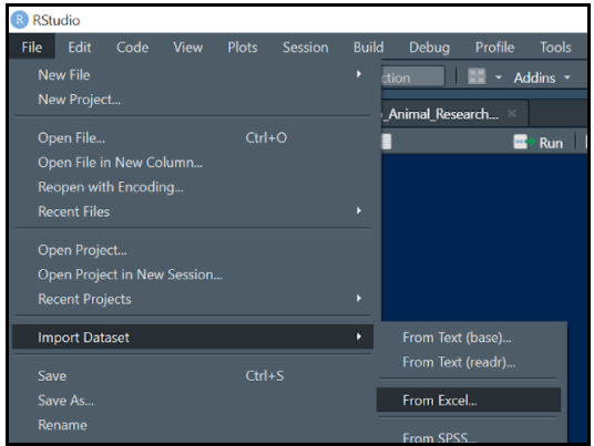
Step 1 – set your working directory! We also need to import our data from an excel file into R Studio using the ‘readxl’ package. If you require a more in-depth tutorial on how to do this refer to the introduction and univariate analysis intensives for R Studio.

Step 2 – We can now shorten our dataset name to make it easier to code further along. To do this we need to use the following code:

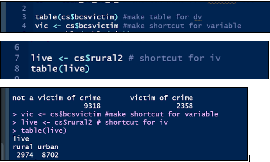
Step 3 – Now we need to produce tables for out two variables, we can also shorten these to make future coding easier also.
To create the table, we need to use the following code:
table (dataset$variable)
To shorten the table command, for future use we need to use the following code:
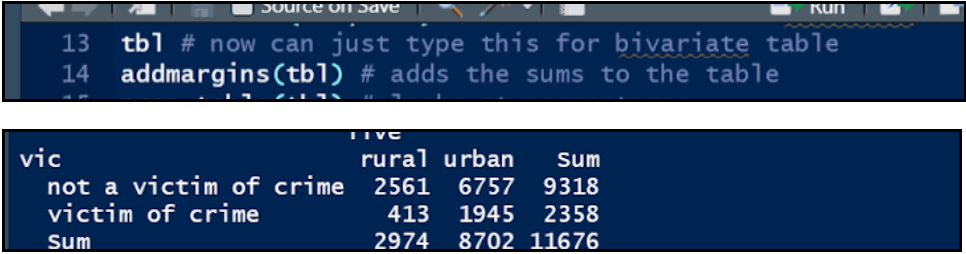
Step 4 – With our shortened variables we can now produce a bivariate table.
Again, we can shorten this to one word using the following code:

This means that every time we type ‘tbl’ it will produce the bivariate crosstab for our variables!
Step 5 – We can now add sums to this table by using:
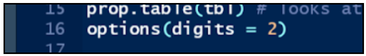
Step 6 – we can change these into percentages or a proportion table using:

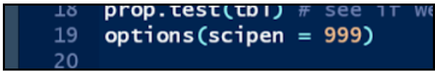
If you would like to reduce the decimal places, we can use the options function like so:
Press ctrl and Ent. Then return to the end of the Code you’d like it applied to, be sure to click and press ctrl+ Ent again.

Step 7 – we can then run a proportion test using a similar code:
To change the p value to a decimal, if it is not already you can use the following code:
Press ctrl and Ent. Then return to the end of the Code you’d like it applied to, be sure to click and press ctrl+ Ent again.
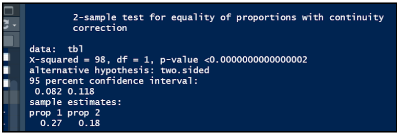
Remember: if this is significant = Fisher’s test, if it is not significant = Chi-Square test
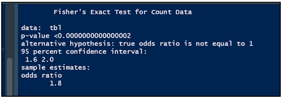
Step 8 – to run the fisher’s test, it is very similar to chi-square we need one piece of code!

Step 9 – If the p value looks like so. You can use:
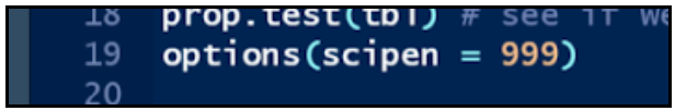
Press ctrl and Ent. Then return to the end of the Code you’d like it applied to, be sure to click and press ctrl+ Ent again.
This makes the value a decimal instead. Round to 3 d.p.
Step 10 – To run a Cramer’s V test. We need to install the ‘lsr’ package. This is a companion package to learning statistics with R Studio! To do this we use the following code:

We can then select it from the packages screen.

After this, we can use the following code to run the test!
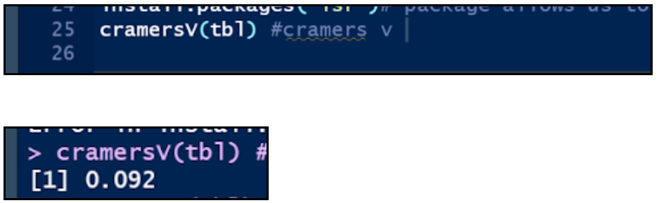
WELL DONE! YOU SUCCESSFULLY PERFORMED A FISHER’S EXACT TEST!