


This guide will walk you through step by step how to conduct a chi-square and Cramer’s V strength of association test using SPSS. This guide may refer to some skills discussed in previous intensives, such as descriptive univariate and bivariate courses. it may be beneficial to complete those first or refer to them if you find yourself struggling.
For this guide we’ll be using a cut down version of the Crime Survey for England and Wales.
Insert link here
Remember: It is always good practice to run Descriptives and clean our data before performing any inferential tests! If you are unsure how to do this, cleaning data and recoding is covered in the univariate analysis RISE intensive, why not give it a go!
For this example, we will be using the following variables:
| DV | bcsvicitm | experience of any crime in the previous 12 months |
| IV | rural | type of area respondent lives in urban/rural |
In Google Sheets, chi square analysis is performed on the tables we create as the user, so we need to create some tables before we can run the test! As Chi-Square compares observed values to the expected values, we need to produce these two tables!
To do this, we first need to produce a pivot table, you should have covered this in earlier intensives, but don’t worry we’ll quickly go through it again!
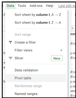
Step 1 – select Data > Pivot table
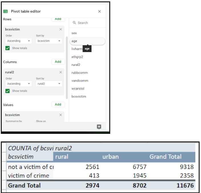
Step 2 – the following box should appear. Ensure the entire dataset is highlighted (this is commonly already done by Google Sheets) and ensure it will be on a new sheet.

Step 3 – It should then take you to a new worksheet, we are going to use the toolbar on the right-hand side (Pivot table editor) to form the pivot table. We need to click our DV in the rows and values boxes and our IV needs to go into the columns box. As shown below.
Now we have our observed counts we need to put these values into a table we have produced ourselves for the chi-square test to work! We can do this under the pivot table on the same worksheet!
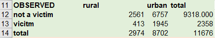
As you can see all of the figures are the same!
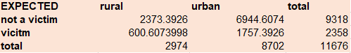
Now we must produce our expected count table, this shows us the counts expected for each category. We are going to do this under the observed count table.
To do this we need to replicate this table with the same headings and totals however, leave the count squares empty.
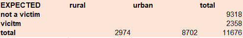
To work out the expected count we can use a formula:
= row total * column total / overall total
This may look confusing so let’s do ‘not a victim’ and ‘rural’ together.
For this one we would use
The row total for that square = 9318 * the column total for that square = 2974 / total count = 11676
Have a go yourself at the rest! You should get a table that looks like the following
We can now finally perform the chi-square test woo!
To do this create a cell that says p value in the cell next to it we are going to input the following formula:
CHISQ.TEST(OBSERVED VALUES, EXPECTED VALUES)
highlight the 4 observed values (not the totals) highlight the 4 expected values (not the totals)
Press Enter and you should get your p value!
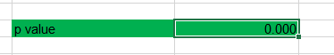
Make sure it is to 3d.p using these buttons.

WELL DONE! YOU SUCCESSFULLY PERFORMED A CHI SQUARE TEST!