


What third variable should I use?
When selecting a third variable to test, it must be an IV, so that we are testing 2 IVs against 1 DV. When running multiple tests, it makes sense to use the IV that produced the largest Cramer’s V to see what difference it makes to the original test. However, as long as you can justify which variable you decide to use, you can use any.
Tip: try not to use a variable with too many categories as this leads to a lot of partial tables, making comparison more difficult and more chance of them being less valid as expected counts < 5 increases.
For this guide we’ll be using a cut down version of the Crime Survey for England and Wales.
Insert link here
We know from the chi-square sprint that our results were significant so let’s use this and add a second IV! In this case let’s see if sex has any effect!
| DV | bcsvicitm | experience of any crime in the previous 12 months |
| IV | rural | type of area respondent lives in urban/rural |
| IV2 | sex | Sex of respondent |
Performing an elaboration in Excel is like performing a Chi-Square, we need to create our own tables again!
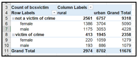
Step 1 – Create a pivot table, instructions on how to do this are in the Chi-Square sprint! The only difference this time is we need to add our third variable. To do this drag sex into the rows field as well as our DV. A warning message may appear, if this happens, select ok.

You should now have a pivot table like so:
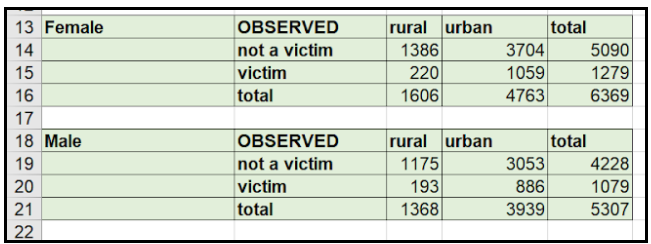
Step 2 – we now need to create our own observed tables using the above pivot table. Just like when performing a chi square, except this time we will be creating two (one for females one for males).
Tip: Read the pivot table carefully if you use the wrong figures this will affect your elaboration!
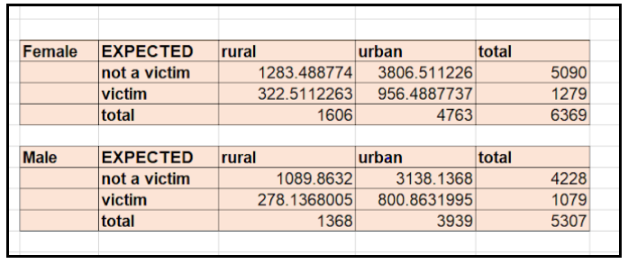
Step 3 – You guessed it, just like Chi-Square we now need to create our expected count tables! Again, there will be two tables (one for females, one for males).
To do this we can copy our observed tables (category names and totals included) . We just need to remove the observed counts for each category so we can replace them with our expected counts.

Apply Your Thinking:
Have a go at the expected counts table, if you need help with the formula refer back to earlier Chi-Square sprints.
The completed expected counts table is below, compare your answers to see if you were right!
To do this were going to use the following formula again:
= row total * column total / overall total
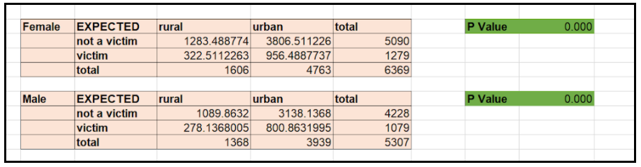
Step 4 – Onto the Chi-Square, this time we are going to perform two! One for each category of our second IV (so one for female and one for male). To do this we again use the same formula:
To do this create a cell that says p value in the cell next to it we are going to input the following formula:

Press Enter and you should get your p value!
WELL DONE YOU CAN NOW PERFORM AN ELABORATION!