


Now we have discovered if there is an association and its significance, we can look at the strength of this association. Remember this is only calculated if the Chi-Square p value is significant.
To do this in Google Sheets, we first need to calculate the chi square value (X²).
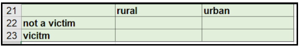
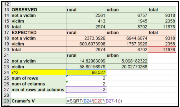
Step 1 – Create a new table underneath your observed count and expected count tables. This table should be similar to your previous crosstab tables but does not need totals.
Step 2 – Next, we need to fill in the four blank cells! To do this, we need to use the following formula:
= (observed count-expected count) ²/ expected count
For example, not a victim x rural. We will be using the observed count and expected count tables previously made.
In this case it would be:
= (2561(observed)-2373.3926(expected)) ²/ 2373.3926(expected)
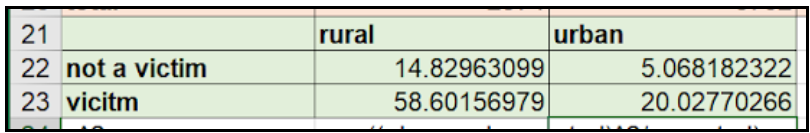
Have a go! The completed table is below if you are stuck or unsure.
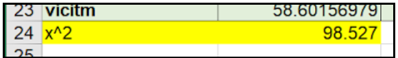
Step 3 – To calculate the Chi-Square Value we then need to find the sum of all these values.
= sum(highlight cells in table)
Now we have figured this value out, we can work on the Cramer’s V formula to work out the strength of the association!
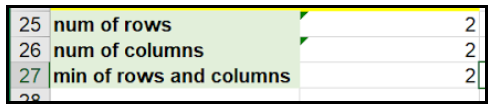
Step 4 – First we need a few details. We need to find the minimum of rows and columns. To do this we need to count the number of rows, the number of columns. We can then use the following formula to find the minimum of these.
= min (num of rows and num of columns)
Step 5 – Now we have all the details to find out our Cramer’s V. Finally! To find this we need to use the formula below.
Cramer’s V = √x2valuegrand total x (of rows and columns-1)
Remember: we now have all of the details for this formula so we can just click the relevant cells!
In this example the formula would have these values:
Cramer’s V = √98.52711676 x 2-1
To do this in google sheets we would type it as:
= sqrt(98.527/(11676 x (2-1)))
All these values can be found in our tables and can just be selected so we don’t have to type in the values!
Remember to close all of the brackets
Step 6 – Press Enter and we should get our strength! We can adjust it to 3 d.p. using the decimal place button shown in the last sprint.
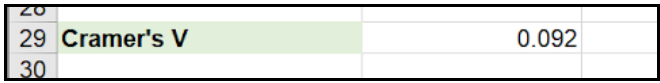
Well Done! You can now perform a Cramer’s V test!