Cleaning Interval and Categorical Data

Cleaning Interval Data

Interval data such as Scale is highly susceptible to outliers, these outliers can then skew your data, we want to avoid this occurring at all costs because outliers can mean we fail to meet the parametric assumptions necessary for certain tests (you’ll be introduced to parametric assumptions in the next intensive). 

We need to identify if we have any outliers present within our data. We will use the variable LifeSat to demonstrate.

Identifying Outliers and Errors. 

Firstly, we can run some commands that will show us our measures of central tendency (MCT) for the variable LifeSat.

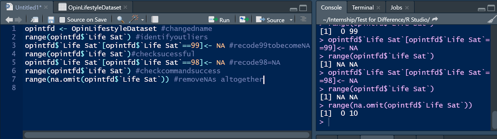
Let’s run a command to find the range: 

range(opintfd$LifeSat) is to be entered. This function will provide us with the minimum and maximum together, you could choose to run some other commands for MCT but this command alone highlights an outlier or skew within the data. 

LifeSat has been measured on a 0-10 scale however as the command showed the min was 0 and maximum 99, we can see there must be an error within our dataset. 

To ensure these errors don’t skew our data and future analysis we need to remove these ‘99s’ and any other errors from our analysis. 

To try and identify all errors we can type in the command View(opintfd) to view our dataset.

Here we can see all of the cases within our dataset. Choosing the blue arrow next to Life Sat we can change our cases to descend, this is shown in the screenshot below. 

A box plot could also be utilised to identify any errors. 

In the above screenshot we can see there are errors or missing codes ‘99’ and ‘98’ included in our Life Sat scale variable, these need to be removed. R Studio doesn’t always automatically code missing values as ‘NA’ as seen in this case, we therefore need to recode these variables so ‘99’ and ‘98’ values become ‘NA’. We would use the commands 

opintfd$`Life Sat`[opintfd$`Life Sat`==99]<- NA

opintfd$’LifeSat’[opintfd$’LifeSat’==98]<- NA

I chose to run each command individually, firstly recoding the ‘99’ in Life Sat to ‘NA’ and checking this was done successfully by inputting another range command for this variable. 

To remove the missing code ‘NA’ from our analysis the command range(na.omit(opintfd$`Life Sat`)) will be used. 

Complete this same process for the ‘98’ values in the Life Sat variable and when both ‘99’ and ‘98’ have been cleaned from our analysis your range should now be 0-10 for this variable. 

The steps above are documented on R in the screenshot below. 

This variable is now ready to use in our analysis!

Cleaning Categorical Data. 

Although you don’t need to worry about outliers within categorical data, errors on the other hand can become quite the nuisance! Cleaning allows us to remove certain answers that are redundant or unhelpful from our analysis without deleting any raw data. 

I would describe redundant responses as categories which do not hold statistical or analytical power, this may be a response that few people have chosen so you decide to remove it from the data, to avoid skewing the overall dataset or a category that wouldn’t provide insight during data analysis, so the decision is made to clean. 

‘Don’t know’ responses may be the best example of this, when a large proportion of your sample have chosen this response it may be wise to keep this category in, the category in itself is posing a unique question, why have so many people chosen don’t know. 

However, when only a few of your sample respondents choose a redundant response often it remains just that, redundant. Ultimately it’s up to you to decide whether a category is an error or not. 

To identify any errors within categorical data the first step is always to run a frequency table/s. There are various different packages and commands that can be used on R Studio to generate a frequency table, these can range from very basic or quite complex. 

My personal favourite is the tabyl function (within the janitor package, make sure this is ticked) as it provides both the counts for each case as well as the percentages for every category within your chosen variable. 

Let’s run a frequency table for the ethnicity variable using the tabyl function.  

tabyl(opintfd$Ethnicity)

Our frequency table for ethnicity is documented below. 

From this screenshot we can see that it makes sense to remove the don’t know response from the ethnicity variable, answers such as these often don’t provide meaningful insight for a number of reasons: 

• ‘Don’t know’ isn’t an ethnicity 
• We don’t know why respondents have answered ‘don’t know’ 
• There is only one person 

This provides a reason to carry out some data cleaning.

We will use the following command to clean the ethnicity variable of the redundant don’t know response. 

Opintfd$Ethnicity[opintfd$Ethnicity==”Don’t know”] <- NA

This code attempts to recode the don’t know response as NA. Running a frequency table using the table function table(opintfd$Ethnicity) we can see Don’t know has been removed/cleaned from our data.