Sampling errors

Sampling Error & Confidence Intervals 

Another step-in data preparation is testing for sampling errors. 

When research is conducted a sample (n) is taken from the wider population (N). Who takes part in the research depends on the sampling technique used. There are many different sampling techniques all with different advantages and disadvantages, statistical testing relies on random sampling techniques. Whilst there are different types of random sampling techniques none are perfect and there is always the potential for anomalies to affect analysis. When this occurs, this can be due to a sampling error  but this is something we can test for before doing our analysis so these errors have limited potential to affect our analysis. 

It’s important to test for sampling errors as these being present in our data could mean we come to a false conclusion during analysis. It could result in us either accepting or rejecting our hypothesis when the opposite is actually true, we could potentially have what is known as: 

Type I error: occurs when a null hypothesis is rejected when its true (false positive) 

OR

Type II error: occurs when the null hypothesis is accepted when it is not true (false negative) 

We need to establish confidence in our sample, that our sample is representative of the wider population. We establish a confidence level by using the following steps. 

To demonstrate these steps, we will continue to use the cut-down version of Opinion Lifestyle Dataset 2015. Using this dataset, we will explore male and female life satisfaction. 

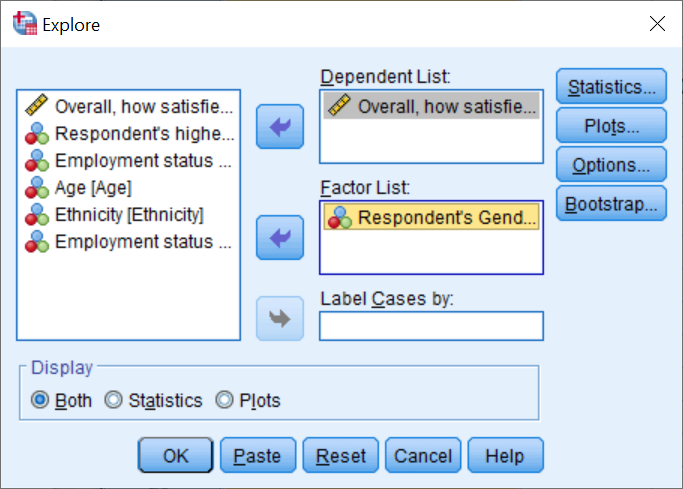
First Select Analyze > Descriptive > Explore. Insert the variables as shown.  

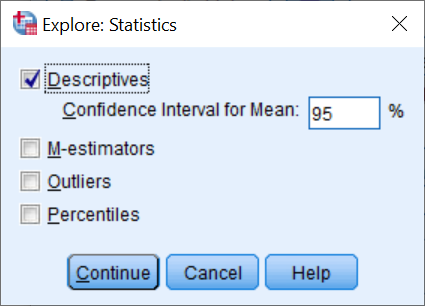
Next select ‘Statistics’ and on doing so a box should pop up, confidence levels should be automatically set as 95% so we don’t need to do anything further here, everything is done automatically. 

Next Select>Plots

In Boxplots, you’ll see ‘Factor levels together’ and ‘stem-and-leaf’ are pre-selected. Leave these, but also tick ‘Normality plots with tests’ as shown in the screenshot above. Select> Continue. 

Whilst a lot of different outputs will pop up, we’re only interested in the ‘Descriptives’ table overleaf and the final output, known as the Box and Whisker plot. Descriptives tells us the confidence intervals for Males and Females (as highlighted below). We want to observe and focus on the mean, and the lower and upper bound 95% confidence interval for mean (for both males and females). 

We can see that for males the mean is 7.64 we have to establish whether we have confidence in this mean. To do this we simply need to look at whether our mean falls within/between the lower and upper bound figures 7.51 and 7.77 respectively. If it does, we can be confident that the mean for men is a ‘true’ mean that is representative of the wider population. 

As we can see we do have confidence in our sample here. We should do the same for females. Looking at the female mean we can see it is 7.69 and falls within the lower and upper bound figures, this means we can be confident in the means as representative of the wider population. 

We also want to make sure our data (for males and females) is from the same sample to test for this we simply review a box and whisker plot. 

If we can draw a line that overlaps the two (or sometimes more) sample groups as shown above, then we can be confident that in this case our two groups are from the same sample.

The boxes indicate the range of scores that go to make up the mean and what our example shows is the difference between the two groups, we can just about see that the female mean is higher than the male mean, this may indicate a gender difference. This is what we would then go on to test. 

How to present your findings… 

‘A review of a box and whisker plot (see figure x) suggested that the data was free from sampling errors. For males, the mean 7.64 (CIs = 7.51-7.77), females, the mean =7.69 (CIs= 7.58-7.81), demonstrating that the mean is representative of the wider population.’ 

1. education and life satisfaction (enter findings below)

2. ethnicity and life satisfaction (enter findings below)